Volumes and Concentrations
droplet_volumes.RmdIn this vignette, calculations to estimate volumes, concentrations and other quantities relevant for the droplet making and picoinjection workflow are documented.
Tubing
Volume of a cylinder with radius \(r\) and height \(h\):
\[V = \pi r^2 h\]
getCylinderVolume <- function(radius, height) {
  return(pi * radius^2 * height)
}
Tubing options
| type | inner diameter | outer diameter |
|---|---|---|
| Tygon | 0.508 mm (0.020 in) | 1.524 mm (0.060 in) |
| PTFE | 0.8 mm | 1.6 mm |
| PTFE | 0.3 mm | 0.78 mm |
# everything in m
radiusTygon <- 0.508e-3 / 2
radiusPTFE <- 0.8e-3 / 2
Plot the tubing volume as a function of tubing length for lengths up to 1 meter:
volumes <- tibble::tibble("length" = seq(1,1000)) %>%
  dplyr::mutate(length = length * 1e-3) %>% # convert into mm
  dplyr::mutate(v_tygon = getCylinderVolume(radiusTygon, length),
                v_ptfe = getCylinderVolume(radiusPTFE, length)) %>%
  tidyr::pivot_longer(c(v_tygon, v_ptfe), names_to = "type", values_to = "volume")
volumes
#> # A tibble: 2,000 × 3
#>    length type      volume
#>     <dbl> <chr>      <dbl>
#>  1  0.001 v_tygon 2.03e-10
#>  2  0.001 v_ptfe  5.03e-10
#>  3  0.002 v_tygon 4.05e-10
#>  4  0.002 v_ptfe  1.01e- 9
#>  5  0.003 v_tygon 6.08e-10
#>  6  0.003 v_ptfe  1.51e- 9
#>  7  0.004 v_tygon 8.11e-10
#>  8  0.004 v_ptfe  2.01e- 9
#>  9  0.005 v_tygon 1.01e- 9
#> 10  0.005 v_ptfe  2.51e- 9
#> # … with 1,990 more rows

ggplot(volumes, aes(x = length, y = volume * 1e9, color = type)) +
  geom_line() +
  scale_colour_viridis_d(labels = c("PTFE", "Tygon")) +
  labs(x = "Tubing length [m]",
       y = "Tubing volume [µL]",
       color = "Tubing type",
       title = "PTFE and Tygon tubing volume") +
  theme_pretty()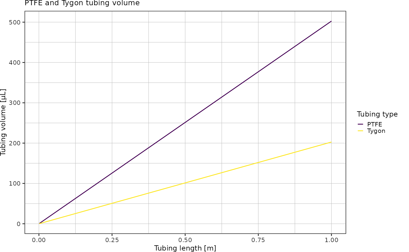
Convert flowrate unit µl/h into tubing cm/h:
flowrates <- tibble::tibble("ul_h" = seq(0, 100)) %>%
  dplyr::mutate("Tygon" = ul_h / (getCylinderVolume(radiusTygon, 0.01) * 1e9),
                "PTFE" = ul_h / (getCylinderVolume(radiusPTFE, 0.01) * 1e9)) %>%
  tidyr::pivot_longer(!ul_h, names_to = "tubing_type", values_to = "cm_h")
ggplot(flowrates, aes(x = ul_h, y = cm_h, color = tubing_type)) +
  geom_line() +
  scale_color_viridis_d() +
  theme_pretty() +
  labs(x = "Flowrate [ul/h]",
       y = "Tubing-length flowrate [cm/h]",
       color = "Tubing type",
       title = "Flowrates in PTFE and Tygon tubing")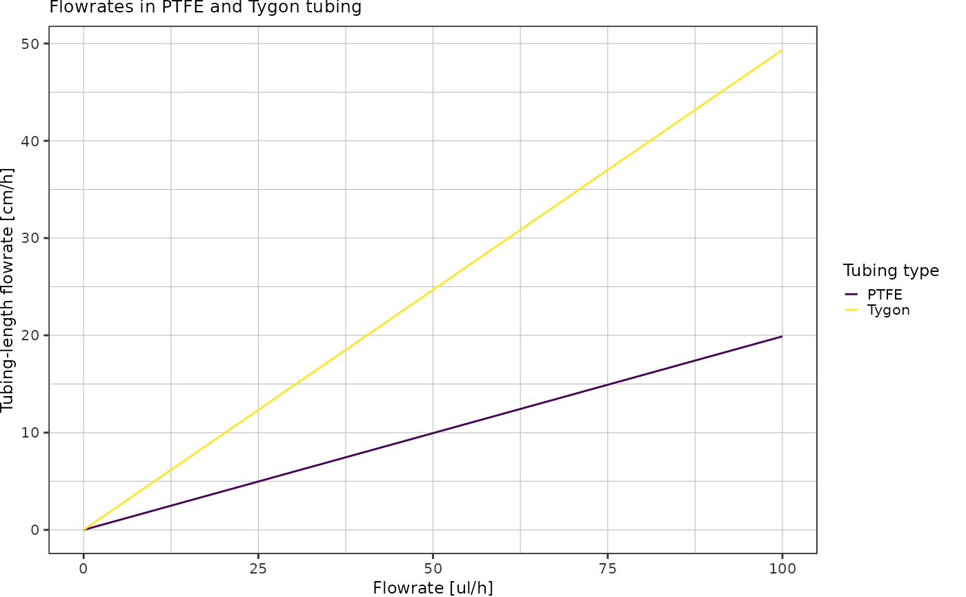
Droplets
How much liquid is contained in a droplet of diameter \(d\)?
Volume of a sphere: \[V = \frac{4}{3} \pi r^3\]
getSphereVolume <- function(radius) {
  return(4/3 * pi * radius^3)
}
Plot droplet volumes as function of diameter:
tibble::tibble("diameter" = seq(10, 100) * 1e-6) %>% # 10-200 µm droplets
  dplyr::mutate("volume" = getSphereVolume(diameter/2)) %>%
  ggplot(aes(x = diameter*1e6, y = volume * 1e15)) + # y-axis in picoliters
  geom_line() +
  labs(x = "Droplet diameter [µm]",
       y = "Droplet volume [pL]",
       title = "Droplet volume vs. diameter") +
  theme_pretty()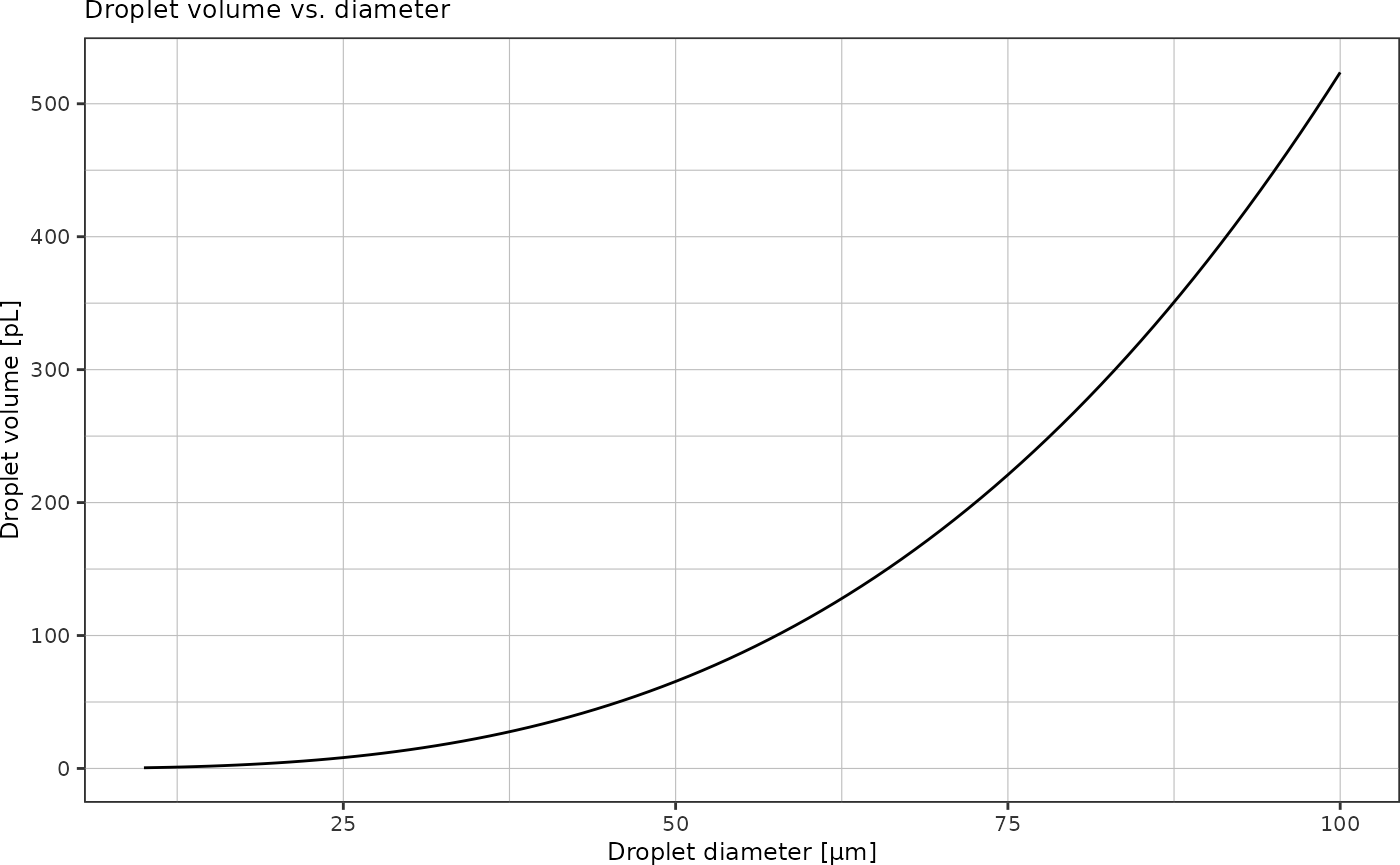
For droplet sizes up to 40 µm:
last_plot() +
  coord_cartesian(xlim = c(10, 40), ylim = c(0, 35))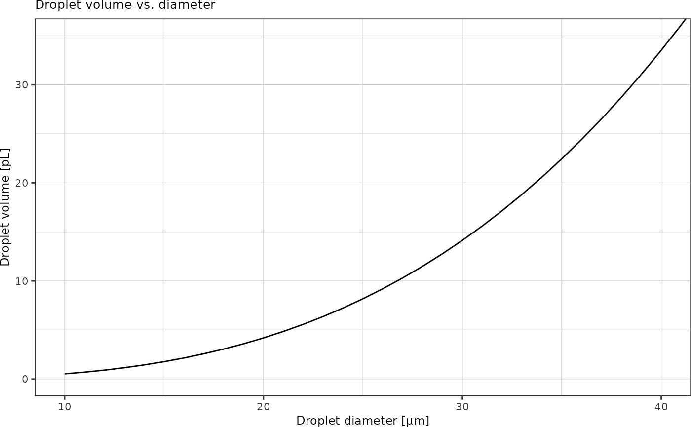
How many droplets are there in x mm of Tygon/PTFE tubing?
radiusDroplet <- 15e-6 # 30 micron dropletsAssuming close-packing of equal spheres: fraction of space occupied by spheres is
\[\frac{\pi}{3 \sqrt{2}} \approx 0.74048\]
Using this packing density, I can calculate the volume occupied by spheres for a given tubing length. Dividing by the known volume of a single droplet yields the total number of droplets contained in x meters of tubing, assuming close-packing of equal spheres.
getNumberOfClosePackedSpheres <- function(radius, volume) {
  volumeSingleSphere <- 4/3 * pi * radius^3
  packingDensity <- pi/3/sqrt(2)
  return(packingDensity * volume / volumeSingleSphere)
}
Plot number of close-packed spheres over tubing length:
volumes %>%
  dplyr::mutate(n_droplets = getNumberOfClosePackedSpheres(radiusDroplet, volume)) %>%
  ggplot(aes(x = length, y = n_droplets*1e-6, color = type)) +
  geom_line() +
  scale_colour_viridis_d(labels = c("PTFE", "Tygon")) +
  labs(x = "Tubing length [m]",
       y = "Number of close-packed spheres [million]",
       color = "Tubing type",
       title = "Number of droplets vs. tubing length") +
  theme_pretty()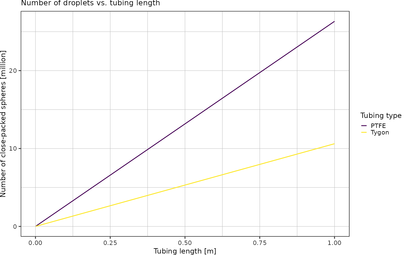
Cells
How does the volume of a cell compare to that of a droplet?
Dimensions of a typical E.coli cell: - diameter = 1 µm - length = 2 µm - volume = 1.3 µm^3
Neglecting the packing, plot how many E.coli cells theoretically fit in one droplet:
vEcoli <- 1.3e-18
tibble::tibble("diameter" = seq(10, 40) * 1e-6) %>% # 10-200 µm droplets
  dplyr::mutate("volume" = getSphereVolume(diameter/2),
                "n_cells" = volume/vEcoli) %>%
  ggplot(aes(x = diameter*1e6, y = n_cells)) + # y-axis in picoliters
  geom_line() +
  labs(x = "Droplet diameter [µm]",
       y = "Number of cells equivalent to droplet volume",
       title = "Number of E.coli cells equivalent to droplet volume vs. droplet diameter") +
  theme_pretty()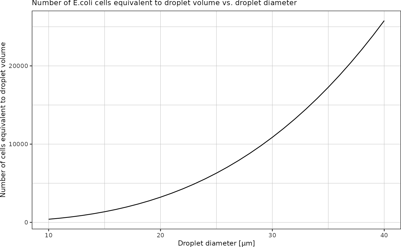
How many mCherry molecules are there in one bacterium, and what is the mCherry concentration in the droplet after cell lysis?
The motivation for this question is the following: In the end, we want to capture those droplets that contained a phage that successfully managed to kill the bacteria. While a droplet containing an intact cell causes a narrow signal of high magnitude after excitation by the laser, a droplet whose cells were lysed should result in a broader, low-intensity signal, since its volumetric concentration of fluorescent protein is much smaller. However, it is not clear, whether this low signal can be distinguished from the background noise that is present at any given time.
Poisson statistics
From (Collins et al. 2015) about single-cell encapsulation:
- when number of encapsulated cells is large and size is significantly
smaller than the droplet (e.g. bacterial cells), the number of cells per
droplet can be representative of the volumetric concentration of cells
- number of cells can be approximated by a Gaussian distribution
- not the case for single-cell analysis
- if cells are distributed randomly in the aqueous phase, the quantity of cells per droplet is determined by Poisson statistics
- probabilistically estimate the proportion of single cells that are encapsulated according to the Poisson distribution, which is applicable in the case where the average cell arrival rate is known and the arrival of individual cells occurs independently from other cells
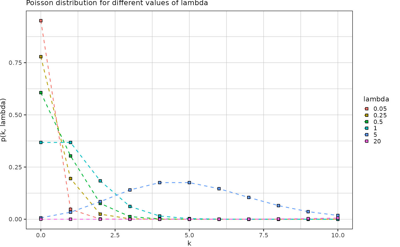
Poisson distribution:
\[p(k, \lambda) = \frac{\lambda^k e^{-k}}{k!}\]
- \(k\) number of particles in a droplet
- \(\lambda\) average number of cells per droplet volume
Plot the Poisson distribution for different \(\lambda\):
tidyr::crossing("k" = seq(0,10),
                "lambda" = c(0.05, 0.25, 0.5, 1, 5, 20)) %>%
  dplyr::mutate("p" = dpois(k, lambda)) %>%
  ggplot(aes(x = k, y = p)) +
  geom_line(aes(color = factor(lambda)), linetype = "dashed") +
  geom_point(aes(fill = factor(lambda)), shape = 22) +
  theme_pretty() +
  labs(title = "Poisson distribution for different values of lambda",
       y = "p(k, lambda)",
       x = "k",
       color = "lambda",
       fill = "lambda")